
MYWAI 4 ROBOTICS AI Algorithms Catalogue
Main functionalities
This module consists of a catalogue of AI algorithms for the analysis of sensory data coming from industrial equipment. In particular, the presented algorithms allow to highlight deviations from standard behaviours and identify recurrent patterns. All the presented algorithms have been tested on triaxial data coming from a series of Inertial Measurement Units (IMUs) attached to a robotic manipulator, but their interfaces are modular, and they can be adapted to other applications or sensors.
In particular the first set of AI algorithms developed and shared enable the intelligent, unsupervised detection of:
- Robotic Joints fault detection
- Robotic Movement pattern searching
- Robotic Multivariate cross related fault detection
Technical specifications
The module groups three different algorithms for the analysis of industrial machinery activities:
- Radial Basis Function Neural Network for fault detection
- Dynamic Time Warping for pattern searching
- Principal Component Analysis for fault detection
Radial Basis Function Neural Network for fault detection
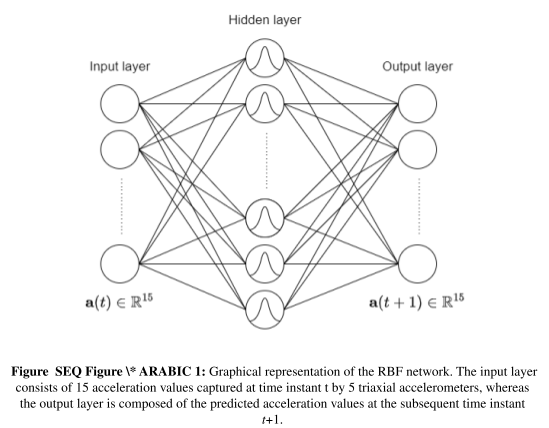
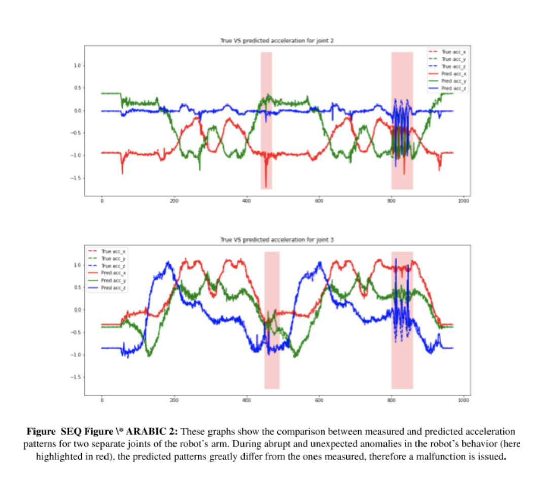
This algorithm is distributed as two functions one to train the Radial Basis Function Neural Network (RBF-NN) and the second one to monitor the machinery behavior. In this algorithm the RBF-NN is used as a regressor to predict the sensor information at the next time instant given the information at the previous time stamp, as depicted in Figure 1. For this reason, it is necessary to train the RBF-NN to correctly predict the sensor information by providing an example of the expected behavior. Therefore, the training function gets as input a multidimensional array containing the sensor data stream and the network parameters (i.e., number of neurons and a value, aka gamma, controlling the level of non-linearity of the radial basis activation function). The sensor array has a dimension of NxL, where L is the number of features (e.g., for a triaxial accelerometer is going to be equal to tree) and N is the number of time stamps collected. Notice that, since the RBF-NN parameters are computed in closed form and only a single repetition of the expected behavior is necessary to train the network, this step is carried out in a very limited amount of time. A vector containing the network parameter resulting from the training process is then saved on file. Similarly, the second function gets as input a multidimensional array, containing the data that should be monitored, a threshold, and loads from file the RBF-NN parameters. The RBF-NN processes each time stamp up to N-1 generating a prediction and matches the prediction with the real value using and Euclidean distances. If for a time stamp the prediction error is higher than the threshold received, that timestamp is reported as an anomaly. Therefore, the module output is binary array of length N-1 specifying if each time stamp presents an anomaly. An example of fault detection applied to the IMU data acquired from the robotic arm is shown in Figure 2.
Dynamic Time Warping for pattern searching
This algorithm is composed of a single function. This function gets as input two multidimensional arrays, one containing data associated to the reference pattern and a second one containing the whole window of data where the search should be performed. Furthermore, the function gets as input two parameters, specified as percentage values: the level of desired correspondence between the reference pattern and possible matches, and a value controlling the overlap between two consecutive windows. Notice that, the higher the overlap value, the more computationally intensive the function becomes, as more iterations of the search are performed, but with a higher accuracy in successfully identifying correspondences.
The reference pattern has a size of NxL, where N is the sample length and L is the number of features. Instead, the second array has a size of MxL, where M is the dimension of the full window on which the search is run. The module inspections the data using a sliding window of length N and uses Dynamic Time Warping (DTW) to measure the distance of the data contained in the windows with the reference pattern. If the distance is under the given threshold (which, in turn, is based on the desired level of correspondence), the window is recognized as a match with the reference pattern. The module returns a binary array of length M where each sample is specified if they belong to the reference pattern or not. Examples of the execution of the presented algorithm are shown in Figure 3 and Figure 4.

Principal Component Analysis for fault detection
This algorithm is composed of a single function. This function gets as input a single multidimensional array containing the data to process, the maximum number of components that the algorithm should consider and a threshold value. The multidimensional array of dimension NxL, where L is the number of features (e.g., for a triaxial accelerometer is going to be equal to tree) and N is the number of time stamps collected, is transformed using the Principal Component Analysis (PCA). PCA is a transformation process for multivariate data usually used for feature reduction. The components computed by the PCA are ranked according to the data variation that they represent. This mechanism implies that, especially when a repetitive behavior is present, the first few principal components represent the behavior while the other contains only noise. We use this mechanism monitoring the last components extracted from the PCA to identify the occurrence of faults. This is performed thresholding the less representative components. Therefore, the module output is binary array of length N specifying if each time stamp presents an anomaly or not. The working mechanism of this algorithm is illustrated in Figure 5 and 6.

Inputs and outputs
Radial Basis Function Neural Network for fault detection
The training function gets as input an NxM array and the network parameters (number of neurons and a value, aka gamma, controlling the level of non-linearity of the radial basis activation function). The training function writes on file the learned network parameters whose size depends on the number of neurons specified. The monitoring function gets as input and NxM array, a threshold and the trained parameters previously saved on file. The monitoring function returns a binary array of length N-1 specifying if each time stamp represents an anomaly or not. Therefore, the function output is binary array of length N specifying if each time stamp presents an anomaly or not.
Dynamic Time Warping for pattern searching
The algorithm gets as input an NxL array representing the pattern thought, an MxL array consisting of the full window of data and two percentage values: correspondence and overlap. Then it returns a binary array of length M specifying if each time stamp belongs to the reference pattern or not.
Principal Component Analysis for fault detection
The algorithm gets as input an NxL array containing the data to monitor, the number of principal components to compute and a threshold. Then it returns a binary array of length N specifying if each time stamp presents an anomaly or not.
Formats and standards
All the algorithms Python implementation uses standard libraries and are available at the following link: https://github.com/TheEngineRoom-UniGe/myway4robotics-repo
Owner (organization)
KNOWHEDGE SRL
UNIVERSITY OF GENOA